
Exadata or not, sometimes Oracle is still Oracle, optimizer is still optimizer, and math is still math.
Here is the story: Instance is Oracle 11.2.0.3, running on an Exadata machine (X2-2 half Rack).
User is complaining query is taking too long to finish (about 5 minutes).
User has also said that last time he run that query, the range scanned was much wider (about a year), nevertheless no performance problems had occurred. Query had finished rather fast the previous time it run… (this is a point to remember for later on).
Let’s look at the query. For the sake of this post, I have simplified it a bit but the idea remains the same.
Basically it is just a simple select, with 4 months range predicates on a date column (SCAN_DATE), and another predicates on some non unique id column (POLICY_NUM).
SELECT COUNT(SCAN_DATE)
FROM my_user.my_table a
WHERE scan_date >= TO_DATE(’01/01/2013 0:0:0′, ‘DD/MM/YYYY HH24:MI:SS’)
AND scan_date < TO_DATE(’01/05/2013 0:0:0′, ‘DD/MM/YYYY HH24:MI:SS’)
AND ( policy_num =’183′ OR policy_num=’000000183′);
Let’s run it and see what happens:
09:51:12 SQL> SELECT COUNT(SCAN_DATE)
FROM my_user.my_table A
WHERE SCAN_DATE >= TO_DATE(’01/01/2013 0:0:0′, ‘DD/MM/YYYY HH24:MI:SS’)
AND SCAN_DATE < TO_DATE(’01/05/2013 0:0:0′, ‘DD/MM/YYYY HH24:MI:SS’)
and ( POLICY_NUM =’183′ OR policy_num=’000000183′);
COUNT(SCAN_DATE)
—————-
0
Elapsed: 00:04:43.87 => NOTICE THE HIGH ELAPSED TIME
Execution Plan
———————————————————-
Plan hash value: 877559244
———————————————————————————————————————————-
| Id | Operation | Name | Rows| Bytes | Cost (%CPU)|Time |
———————————————————————————————————————————-
| 0 | SELECT STATEMENT | | 1 | 16 | 7 (0)| 00:00:01 |
| 1 | SORT AGGREGATE | | 1 | 16 | | |
|* 2 | TABLE ACCESS BY INDEX ROWID | MY_TABLE | 1 | 16 | 7 (0)| 00:00:01 |
|* 3 | INDEX RANGE SCAN | SCAN_DATE_INDX | 9 | | 3 (0)| 00:00:01 |
———————————————————————————————————————————-
Predicate Information (identified by operation id):
—————————————————
2 – filter(“POLICY_NUM”=’000000183′ OR “POLICY_NUM”=’183′)
3 – access(“SCAN_DATE”>=TO_DATE(‘ 2013-01-01 00:00:00’, ‘syyyy-mm-dd hh24:mi:ss’)
AND “SCAN_DATE”<TO_DATE(‘ 2013-05-01 00:00:00’, ‘syyyy-mm-dd hh24:mi:ss’))
Statistics
———————————————————-
1 recursive calls
0 db block gets
4622469 consistent gets => NOTICE THE HIGH CONSISTENT GETS
375620 physical reads => AND HIGH PHYSICAL READS
8320 redo size
533 bytes sent via SQL*Net to client
520 bytes received via SQL*Net from client
2 SQL*Net roundtrips to/from client
0 sorts (memory)
0 sorts (disk)
1 rows processed
The above execution plan is showing index range scan is used (bolded line). It is also stated in the plan thatoptimizer thinks only 9 rows will be returned by the index. This looked suspicious to me, since table has millions of rows.
Let’s view the execution in OEM SQL Monitoring (this is a great and most recommended feature!!!).
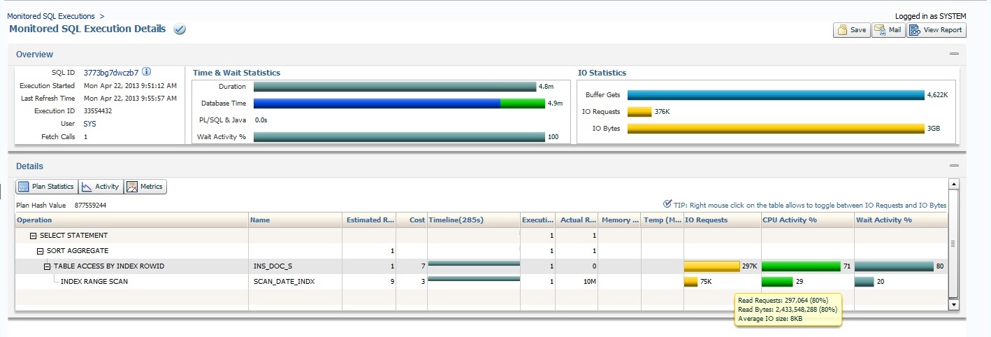
Indeed it shows that although estimated rows is 9 (and this is what making the optimizer wrongly choose his decision), the actual returned rows are 10M.
Exadata or not Exadata, optimizer is still optimizer, and math is still math.
Scanning 10M rows through an index is obviously not the best thing to do (and this is an understatement).
Just think about it. Even if IO latency is very very good, lets say 0.5ms (which is considered to be very good latency for random reads), multiplying 0.5ms by 10M seeks will still take forever.
So what is making Oracle choose a wrong decision?
10:21:32 SQL> select num_rows,last_analyzed
from dba_tables
where owner=’MY_OWNER’
and table_name=’MY_TABLE’;
NUM_ROWS LAST_ANAL
—————— —————–
168,562,490 26-OCT-12
Table was last analyzed on 26.10.2012? Six months ago? This doesn’t sound promising. But let’s continue and look what are the statistics of those two relevant columns, especially low value and high value..
(btw, I have simplified the select on the low/high_value to make the query below more readable and short. To be able to see the real values on these two column you need to use some conversion on it.)
10:28:29 SQL> SELECT column_name,data_type,num_distinct,density,last_analyzed,low_value,high_value
10:28:29 18 from DBA_TAB_COLUMNS a
10:28:29 19 where table_name=’MY_TABLE’
10:28:29 20 and column_name in (‘POLICY_NUM’,’SCAN_DATE’);
COLUMN_NAME DATA_TYPE NUM_DISTINCT DENSITY LAST_ANAL LOW_V HI_V
————— ———- ———— ———- ——— ———- ——————– ——————–
POLICY_NUM VARCHAR2 3922917 5.1066E-06 26-OCT-12 8888
SCAN_DATE DATE 19276420 .00002758 26-OCT-12 1981-1-1 0:0:0 2012-10-22 2:51:48
Look what we found. The highest value of SCAN_DATE column is 22.10.2012. Obviously this is because last time table was analyzed was in 26.10.2012. No wonder Oracle thought there won’t be many rows returned for the requested predicate. The requested predicate is requesting rows when scan date between 1.1.2013 – 1.5.2013. This date range is higher thna the high_value of scan_date column:
WHERE SCAN_DATE >= TO_DATE(’01/01/2013 0:0:0′, ‘DD/MM/YYYY HH24:MI:SS’)
AND SCAN_DATE < TO_DATE(’01/05/2013 0:0:0′, ‘DD/MM/YYYY HH24:MI:SS’)
Now let’s see how many rows are actually in the table. Notice the hints I have used, and how fast Oracle returned the result. Those hints are forcing Oracle to use index fast full scan with parallel query (degree 4), which is much more appropriate in this case than a simple index range scan, since table has millions of rows (Note: Exadata offloadingis also relevant here, and I have added a special section for that at the end of this post).
10:04:49 SQL> SELECT /*+ index_ffs (a,scan_date_indx) parallel_index(a,scan_date_indx,4) */
COUNT(SCAN_DATE)
FROM my_owner.my_table A;
COUNT(SCAN_DATE)
—————-
186,863,326
Elapsed: 00:00:05.44
Table has 186M rows. Now let’s see how many rows will be returned for the requested dates:
10:05:11 SQL> SELECT /*+ index_ffs (a,scan_date_indx) parallel_index(a,scan_date_indx,4) */ COUNT(SCAN_DATE)
FROM my_owner.my_table A
WHERE SCAN_DATE >= TO_DATE(’01/01/2013 0:0:0′, ‘DD/MM/YYYY HH24:MI:SS’)
and scan_date < to_date(’01/05/2013 0:0:0′, ‘DD/MM/YYYY HH24:MI:SS’);
COUNT(SCAN_DATE)
—————-
10,213,081
Elapsed: 00:00:04.95
Indeed, 10M rows are returned here. This is not a surprise, since we have already seen the huge gap between estimated rows and actual rows in OEM’s SQL Monitoring screen.
Here is the time to say that after finding there is a statistics problem here, I have explored the issue a bit more with the customer, to figure out what was the case when query run much faster (remember this was part of the complaint?). It appeared that query run much faster when the rows were selected from year 2012. Customer has informed me that since they started running the query on year 2013, query was taking forever..
And now we know why..
Let’s explore it a bit more, and see how many rows are returned for 2012:
10:06:07 SQL> SELECT /*+ index_ffs (a,scan_date_indx) parallel_index(a,scan_date_indx,4) */ COUNT(SCAN_DATE)
10:06:07 2 FROM my_owner.my_table A
10:06:07 3 WHERE SCAN_DATE >= TO_DATE(’01/01/2012 0:0:0′, ‘DD/MM/YYYY HH24:MI:SS’)
10:06:07 4 and scan_date < to_date(’01/05/2012 0:0:0′, ‘DD/MM/YYYY HH24:MI:SS’);
COUNT(SCAN_DATE)
—————-
10,381,170
Elapsed: 00:00:04.24
Let’s see what Oracle thinks about the cardinality of this predicate:
10:07:16 SQL> SELECT /*+ index_ffs (a,scan_date_indx) parallel_index(a,scan_date_indx,4) */ COUNT(SCAN_DATE)
10:07:16 2 FROM my_owner.my_table A
10:07:16 3 WHERE SCAN_DATE >= TO_DATE(’01/01/2012 0:0:0′, ‘DD/MM/YYYY HH24:MI:SS’)
10:07:16 4 and scan_date < to_date(’01/05/2012 0:0:0′, ‘DD/MM/YYYY HH24:MI:SS’);
COUNT(SCAN_DATE)
—————-
10381170
Elapsed: 00:00:04.01
Execution Plan
———————————————————-
Plan hash value: 1948420453
———————————————————————————————————————————
| Id | Operation | Name | Rows | Bytes | Cost (%CPU)| Time | TQ |IN-OUT| PQ Distrib |
———————————————————————————————————————————
| 0 | SELECT STATEMENT | | 1 | 7 | 155K (1)| 00:31:05 | | | |
| 1 | SORT AGGREGATE | | 1 | 7 | | | | | |
| 2 | PX COORDINATOR | | | | | | | | |
| 3 | PX SEND QC (RANDOM) | :TQ10000 | 1 | 7 | | | Q1,00 | P->S | QC (RAND) |
| 4 | SORT AGGREGATE | | 1 | 7 | | | Q1,00 | PCWP | |
| 5 | PX BLOCK ITERATOR | | 9473K| 63M| 155K (1)| 00:31:05 | Q1,00 |PCWC||
|* 6 | INDEX STORAGE FAST FULL SCAN| SCAN_DATE_INDX | 9473K| 63M| 155K (1)| 00:31:05 | Q1,00 | PCWP | |
———————————————————————————————————————————
Predicate Information (identified by operation id):
—————————————————
6 – storage(“SCAN_DATE”>=TO_DATE(‘ 2012-01-01 00:00:00’, ‘syyyy-mm-dd hh24:mi:ss’) AND “SCAN_DATE”<TO_DATE(‘
2012-05-01 00:00:00’, ‘syyyy-mm-dd hh24:mi:ss’))
filter(“SCAN_DATE”>=TO_DATE(‘ 2012-01-01 00:00:00’, ‘syyyy-mm-dd hh24:mi:ss’) AND “SCAN_DATE”<TO_DATE(‘
2012-05-01 00:00:00’, ‘syyyy-mm-dd hh24:mi:ss’))
Statistics
———————————————————-
12 recursive calls
108 db block gets
588111 consistent gets
585699 physical reads
0 redo size
537 bytes sent via SQL*Net to client
520 bytes received via SQL*Net from client
2 SQL*Net roundtrips to/from client
0 sorts (memory)
0 sorts (disk)
1 rows processed
As expected, when the given date range is for 2012 (i.e SCAN_DATE >= TO_DATE(’01/01/2012 0:0:0′, ‘DD/MM/YYYY HH24:MI:SS’) and SCAN_DATE < to_date(’01/05/2012 0:0:0′, ‘DD/MM/YYYY HH24:MI:SS’) ),
the estimated returned rows Oracle is showing (9473K) is much more accurate.
And why does the query returns much faster when the given date range was for 2012?
Because Oracle knows scanning this index will bring 10M rows, so it smartly decides not to use this index. Instead, it uses the index on POLICY_NUM, as shown below.
Notice also the monitor hint. This will enable us to view the execution in SQL Monitoring, since by default, only long running queries (above 5 seconds) or parallel queries are shown.
09:49:11 SQL> set autotrace on
09:49:34 SQL>
09:49:46 SQL> SELECT /*+ monitor */ COUNT(SCAN_DATE)
09:49:47 2 FROM my_owner.my_table A
09:49:47 3 WHERE SCAN_DATE >= TO_DATE(’01/01/2012 0:0:0′, ‘DD/MM/YYYY HH24:MI:SS’)
09:49:47 4 AND SCAN_DATE < TO_DATE(’01/05/2012 0:0:0′, ‘DD/MM/YYYY HH24:MI:SS’)
09:49:47 5 and ( POLICY_NUM =’183′ OR policy_num=’000000183′);
COUNT(SCAN_DATE)
—————-
0
Elapsed: 00:00:00.01
Execution Plan
———————————————————-
Plan hash value: 1090044264
————————————————————————————————-
| Id | Operation | Name | Rows | Bytes | Cost (%CPU)| Time |
————————————————————————————————-
| 0 | SELECT STATEMENT | | 1 | 16 | 62 (0)| 00:00:01 |
| 1 | SORT AGGREGATE | | 1 | 16 | | |
| 2 | INLIST ITERATOR | | | | | |
|* 3 | TABLE ACCESS BY INDEX ROWID| MY_TABLE | 4 | 64 | 62 (0)| 00:00:01 |
|* 4 | INDEX RANGE SCAN | INDX_POLICY_NUM | 79 | | 4 (0)| 00:00:01 |
————————————————————————————————-
Predicate Information (identified by operation id):
—————————————————
3 – filter(“SCAN_DATE”>=TO_DATE(‘ 2012-01-01 00:00:00’, ‘syyyy-mm-dd hh24:mi:ss’) AND
“SCAN_DATE”<TO_DATE(‘ 2012-05-01 00:00:00’, ‘syyyy-mm-dd hh24:mi:ss’))
4 – access(“POLICY_NUM”=’000000183′ OR “POLICY_NUM”=’183′)
Statistics
———————————————————-
1 recursive calls
0 db block gets
8 consistent gets
3 physical reads
0 redo size
533 bytes sent via SQL*Net to client
520 bytes received via SQL*Net from client
2 SQL*Net roundtrips to/from client
0 sorts (memory)
0 sorts (disk)
1 rows processed
So the only question remains open is why does statistics are not updated, as this is an Oracle 11.2.0.3 instance, and statistics gathering through dbms_stats should be done automatically.
I suspected locked statistics. Let’s check that:
10:08:41 SQL> select owner, table_name, stattype_locked
from dba_tab_statistics
where table_name=’MY_TABLE’ ;
OWNER TABLE_NAME STATTYPE_LOCKED
———- ————— ————————-
IMAGE MY_TABLE ALL
As suspected, statistics are locked!!! No wonder last time table was analyzed was 6 months ago. For date fields, this is a bad thing. You can lock statistics if and only if it has no effect the optimizer decision. And clearly this is not the case here. Optimizer decision was effected becuase high_value on the date column had a wrong value (much lower value than it should).
Resolution here is simple. Unlock statistics, re-gather statistics, and… Voilà!! . Query “suddenly” runs much faster…
Let’s see what happens to “high_value” statistics, after unlocking and re-gathering statistics on MY_TABLE:
12:41:32 SQL> SELECT owner,column_name,data_type,num_distinct,density,last_analyzed,num_nulls,
low_value,high_value
from DBA_TAB_COLUMNS a
where table_name=’MY_TABLE’
and column_name in (‘POLICY_NUM’,’SCAN_DATE’);
COLUMN_NAME DATA_TYPE NUM_DISTINCT DENSITY LAST_ANAL NUM_NULLS LOW_V HI_V
————— ———- ———— ———- ——— ———- ——————– ——————–
POLICY_NUM VARCHAR2 5634560 9.9753E-06 28-APR-13 0 8888
SCAN_DATE DATE 5644288 0 .000045952 28-APR-13 0 1981-1-1 0:0:0 2013-4-28 12:1:31
Brilliant. HIGH_VALUE now has the correct value, so let’s re-run the original query and see how Oracle execute it this time:
12:42:21 SQL> SELECT COUNT(SCAN_DATE)
FROM my_owner.my_table A
WHERE SCAN_DATE >= TO_DATE(’01/01/2013 0:0:0′, ‘DD/MM/YYYY HH24:MI:SS’)
AND SCAN_DATE < TO_DATE(’01/05/2013 0:0:0′, ‘DD/MM/YYYY HH24:MI:SS’)
and ( POLICY_NUM =’183′ OR policy_num=’000000183′);
COUNT(SCAN_DATE)
—————-
0
Elapsed: 00:00:00.01
Execution Plan
———————————————————-
Plan hash value: 1090044264
————————————————————————————————-
| Id | Operation | Name | Rows | Bytes | Cost (%CPU)| Time |
————————————————————————————————-
| 0 | SELECT STATEMENT | | 1 | 18 | 52 (0)| 00:00:01 |
| 1 | SORT AGGREGATE | | 1 | 18 | | |
| 2 | INLIST ITERATOR | | | | | |
|* 3 | TABLE ACCESS BY INDEX ROWID | MY_TABLE | 3 | 54 | 52 (0) | 00:00:01 |
|* 4 | INDEX RANGE SCAN | INDX_POLICY_NUM | 61 | | 5 (0) | 00:00:01 |
————————————————————————————————-
Predicate Information (identified by operation id):
—————————————————
3 – filter(“SCAN_DATE”>=TO_DATE(‘ 2013-01-01 00:00:00’, ‘syyyy-mm-dd hh24:mi:ss’) AND
“SCAN_DATE”<TO_DATE(‘ 2013-05-01 00:00:00’, ‘syyyy-mm-dd hh24:mi:ss’))
4 – access(“POLICY_NUM”=’000000183′ OR “POLICY_NUM”=’183′)
Statistics
———————————————————-
0 recursive calls
0 db block gets
8 consistent gets
0 physical reads
0 redo size
533 bytes sent via SQL*Net to client
520 bytes received via SQL*Net from client
2 SQL*Net roundtrips to/from client
0 sorts (memory)
0 sorts (disk)
1 rows processed
Excellent. As expected, after Oracle sees the right statistics, it now knows the highest value for SCAN_DATE is 28.4.13 and not 26.10.12, therefore it can smartly choose much more suitable execution plan. This time Oracle decides not to range scan the index SCAN_DATE_INDX (since it knows such range will be wide), but instead, it chooses to range scan INDX_POLICY_NUM.
This time the result is returned in no time.
Oracle is no mystery. Just need to understand it, and know how it works.
🙂
And now, if you can just bare with me a bit longer, here is some cool exadata staff to notice:
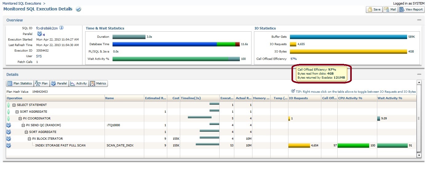
Since we forced an index fast full scan with parallel, Oracle was able to use Exadata smart scan offloading (btw, to enable the possibility of smart scan use, full scan and direct read are a must). Since the only column used in this query is scan_date, offloading is extremely effective here: more than 4GB were offloaded (i.e database didn’t need to process those 4G as most of them were already filtered by the storage). This can also be seen in OEM, as “cell offload efficiency: 97%”:
This smart scan can be also verified through v$sesstat:
SQL> select b.name,a.value from v$sesstat a, v$statname b, v$session c
where a.statistic# = b.statistic#
AND A.SID=C.SID
AND ( B.NAME like ‘%storage%’ or b.name like ‘%offload%’)
and a.sid=1542
order by a.value desc;
NAME VALUE
—————————————————————- ———-
cell physical IO bytes eligible for predicate offload 0
cell simulated physical IO bytes returned by predicate offload 0
cell simulated physical IO bytes eligible for predicate offload 0
cell physical IO bytes saved by storage index 0
Notice that before running the query, “cell physical IO bytes eligible for predicate offload” is 0.
Now, let’s run the query again.
SQL> SELECT /*+ index_ffs (a,scan_date_indx) parallel_index(a,scan_date_indx,4) */ COUNT(SCAN_DATE)
2 FROM IMAGE.INS_DOC_S A
3 WHERE SCAN_DATE >= TO_DATE(’01/01/2012 0:0:0′, ‘DD/MM/YYYY HH24:MI:SS’)
4 and scan_date < to_date(’01/05/2012 0:0:0′, ‘DD/MM/YYYY HH24:MI:SS’);
COUNT(SCAN_DATE)
—————-
10381208
Now let’s see if statistics values have changed:
SQL> select b.name,a.value from v$sesstat a, v$statname b, v$session c
where a.statistic# = b.statistic#
AND A.SID=C.SID
AND ( B.NAME like ‘%storage%’ or b.name like ‘%offload%’)
and a.sid=1542
order by a.value desc;
NAME VALUE
—————————————————————- ———-
cell physical IO bytes eligible for predicate offload 4798046208
cell simulated physical IO bytes eligible for predicate offload 0
cell simulated physical IO bytes returned by predicate offload 0
cell physical IO bytes saved by storage index 0
After we execute the query, “cell physical IO bytes eligible for predicate offload” had jump to 4798046208. Meaning, smart scan did happen, and this offload is all due to this query.
Cool and effective!
🙂
That’s all for now. Hope you’ve enjoyed this post.
As always, comments are most welcomed.
Merav Kedem,